Where gain smoothing and correction has gone badly awry, the Xenon line will no longer appear at 29.6 keV. You may be able to check this in your own data by making a detector spectrum that includes all the counts from the shadowgram, including the instrument background.
It must be stressed that the absolute correctness of the gain correction of a particular Science Window or Revolution, cannot be determined until a full Xe line analysis of all the SCWs in a revolution has been performed. Even when a gain history table is smoothed properly, and the fit to the raw gain is good circumstances can arise that affect the gain on the detector plate without showing up in the calibration spectra (See `Hidden Gain Variation Problems' below). The JEM-X team endeavours to perform a Xe-line analysis and create IC tables before the consolidated processing of the data, though this was not always possible in the past.
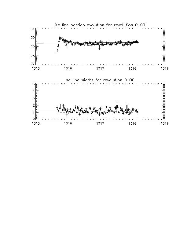
A clear example of a well-corrected revolution is revolution 100, JEM-X2, where after a rocky start due to the usual spatial gain variation changes found at the beginning of every revolution, the Xe line position settles down to a value very close to 29.6 keV. See below for more on problems at the beginning of each revolution.
If there is a known problem with the gain calibration of one of the units, then a corrected gain history table will be delivered to ISDC by the JEM-X team. These corrected tables are determined offline by the team, and stored at ISDC as Instrument Characteristics tables. If there is an IC gain history table for a particular revolution (only a few revolutions have these prior to revolution 900), then the OSA software from OSA 6.0 onwards will use these tables automatically instead of the gain history table derived by the ISDC pipeline.
A quick glance through the Gain Calibration link table will show you that the vast majority of the revolutions processed are well-behaved and well-processed, prior to revolution 900. However, those lines with pink/red or green backgrounds indicate revolutions with some gain calibration problem. After revolution 949 every revolution must be processed using an IC table due to non-linear temperature effects, instrument aging of the microstrip plate and decay in intensity of the calibration sources.
Pink and red colours indicate revolutions which still have problems even using the latest software. The darkness of the colour indicates the severity of the problem. Pale pink can mean that an entire revolution is affected very slightly, possibly to an extent not even noticeable to the uninitiated, or it could indicate a noticeable problem for a small part of the revolution. These problems are now covered by the delivery of IC tables to ISDC.
Shades of green indicate revolutions that had problems being processed with old versions of the software, most notably, sparse gain history tables produced using j_calib_gain_fitting 7.1. However, with newer software these problems are corrected. It is important for some revolutions, usually those with heavy grey filtering, that the gain history table is generated with verion 7.2 not 7.1. This is not easy for the non-specialist to determine. Be sure to download the latest revolution file data before you begin processing, and start the JEM-X Science Analysis at level COR.
Corrected science data is archived in the ISDC repositories, but this is invariably a reflection of the processing as it was a year or more ago. If you want the best possible results, be sure to have the latest instrument characteristics tables, the most recently generated revolution files, the latest version of the Offline Science Analysis (OSA) software and start all you processing at analysis level COR.
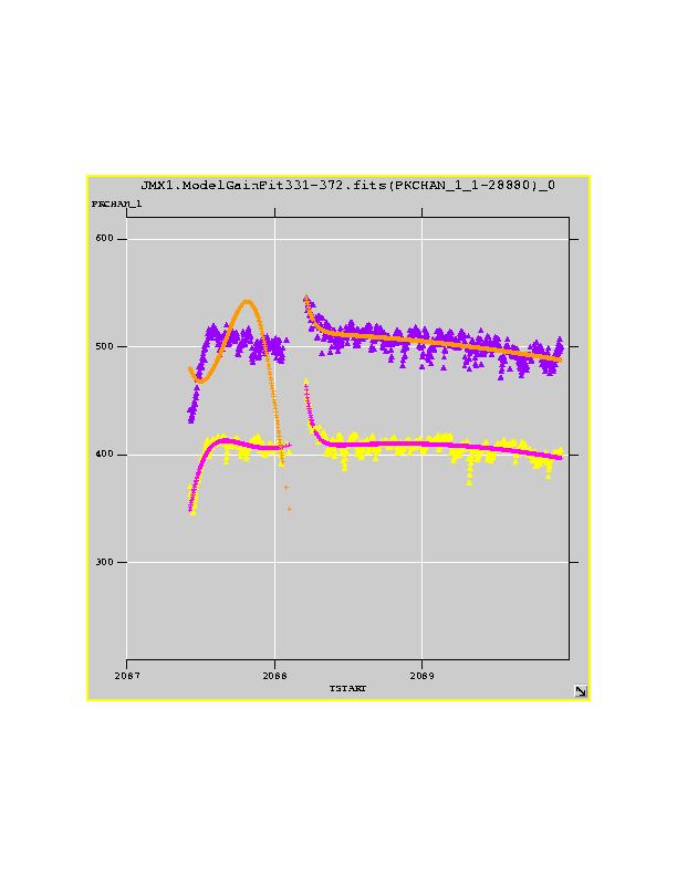
A Good example of automatic gain fitting gone awry can be seen for JEM-X1 in revolution 358. In this case, a telemetry glitch immediately before an emergency switch off has resulted in a spurious gain history point for the last calibration source polled by the onboard software, resulting an a Cd position of PHA=95. This data point cannot even be seen on the plot, but its effect is clear. The smoothed line takes a graceful dive downwards that will result in energy values for the first part of the revolution that are either slightly too low (smoothed curve lies slightly above the raw data) or far too high (smoothed curve lies far below the raw data). The solution is to make sure that you have the latest instrument characteristics tables which OSA version 6.0, and later versions, can use to correct these problems.
In a very small number of unusual cases we have discovered that the gain on the detector plate is not always mirrored by the calibration source spectra that we use for gain correction. One of the best examples of this problem, though slight and short-lived, is revolution 276. While this sort of gain suppression might happen in any circumstances where there is high background activity (and hence plate charging), the example of revolution 332 is still unique in the mission, and still not really understood.
Evidently the only cure for these problems is to use the IC gain history tables developed after offline analysis by the JEM-X team and delivered to ISDC as Instrument Characteristics (IC) files.
During perigee passage, the high voltage (HV) supply to the detector plates of the JEM-X instruments is switched off to protect the instruments from being bombarded by particles in the radiation belts. During these periods (and other longer periods of dormancy) the ion migration in the detector plates relaxes and the units revert towards their launch values of both gain and spatial gain variations. On reactivation, each unit takes some time to re-establish its current degree of ion migration and gain.
For a standard perigee passage this will take a couple of hours as in the case of JEM-X2, revolution 100, shown above. For a switch off of a revolution or more the effect may be seen for considerably longer, for example revolution 239 where JEM-X2 is switched on for the Crab calibration exercises.
While the units are recovering their gain configuration, it is not just the gain of the instrument detector plate as a whole that is changing, but the spatial gain variations (SPAG) which are usually desribed by the SPAG-MOD table in the Instrument Model. Unfortunately during this recovery process, the SPAG-MOD table does not describe the instantaneous gain variations of the plate. During these periods both the degree and speed of SPAG changes varies all over the plate and cannot be mapped because it also depends strongly on the length of time the unit has been de-activated before switch on.
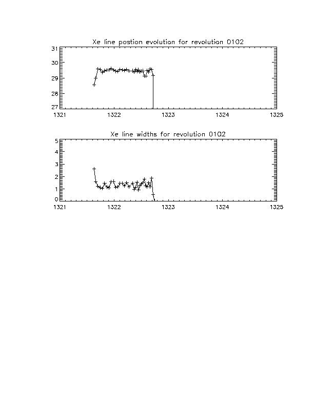
Consequently, the gain correction cannot be performed perfectly for these periods, and we see both a drop in the Xe line position from 29.6 keV and a broadening of the gaussians fitted to the line for each Science Window. The best example of this effect can be seen on JEM-X2 revolution 102.
The instrument team is looking into the possiblity of maintaining a lowered HV supply to the instrument plates during perigee passage to minimize the amount of time spent on gain recovery. Exercises conducted during Crab calibration suggest that this could indeed help reduce the problem.
For reactivation of either unit after a long dormant period (i.e. JEM-X2 from revolutions 170 to 856 and JEM-X1 from 856 to 976) when only one unit was being run on a daily basis, there was such a marked change in both average instrument gain and local SPAG (spatial gain variation) that these warm-up periods are covered by their own BTIs. Although the Xe line position can appear quite good during these periods, other recovered values like fluxes may well be affected by the unmeasureable gain changes across the microstrip plate, and the upper and lower electronic cutoffs that sort out particles from real X-ray events.
If possible find the Xe line in the detector background spectra of your data to assess how well gain correction has proceeded, or better still, take a look at the Xe line evolution of the entire revolution if it is available on this site. I add new analyses to the site almost every day. Also read the notes on the revolution - these are also added and updated regularly.
Do not read too much into small energy changes in your favourite emission lines etc. if these same changes are reflected in the xenon line of the same data. Treat the first few Science Windows in every revolution, or after unplanned switch offs, with caution if energy determination is particularly important to you. If in doubt about the reliablity of your spectral or energy data, you are welcome to contact the JEM-X team for help.
CAO 09/02/2011