Absolute Gravimetry with Quantum Technology
Tim Enzlberger Jensen, DTU Space
Table of Contents
Introduction
The gravity acceleration, $\bf{g}$, is a vector quantity characterized by both magnitude, $g = \vert\bf{g}\vert$, and direction, $\hat{\bf{g}}$. Absolute gravity measurements usually focus on determining only the magntiude, $g$. Historically, there have been two approaches both introduced by Galileo Galilei around 1600:- The pendulum method
- The free-fall method
where $T$ is the period of oscillation and $l$ is the length of the pendulum. In reality the pendulum is affected by friction and air drag, making such a simple gravity pendulum difficult to realize. Nonetheless, the pendulum approach was the dominant method for around 300 years. Moreover, in 1656 Christian Huygens build the first pendulum clock, which was a great improvement compared to the existing mechanical clocks. In 1671, Jean Richer brought such a pendulum clock on an expedition to French Guiana and found the number of swings per day different than in France. This indicated that gravity was not constant around the globe and sparked a great debate over the shape of the Earth, which was at that point believed to be perfectly spherical. Today, the most common choice for absolute gravimeters is the free-fall method. The underlying principle that the acceleration of a freely falling body is independent of its mass was also proposed by Galileo Galileo with his famous experiments tossing objects off the leaning tower of Pisa between 1589 and 1592. In a homogenous gravity field, the path of a falling object is governed by the equation:
where $z$ is the position while $z_0$ and $\dot{z}_0$ represents the position and velocity at the starting time of the experiment, i.e. at $t=0$. This indicates that if the position, $z_n$, can be measured at several instances in time, $t_n$, a curve of the form above can be fitted to the data and the gravity acceleration can be derived. This concept is illustrated in the animation below.
Essentially, both methods introduced above relates to the determination of the fundamentatal concepts of length and time. For the precise determination of both of these, quantum technology has already contributed with essential technology, i.e. lasers and atomic clocks, which are fundamental in modern gravimeters such as the Micro-g LaCoste FG5. Such gravimeters are however not referred to as "Quantum Gravimeters". Instead we talk about a first and second quantum revolution. One might thus say that both modern "classical" gravimeters and quantum gravimeters are based on principles of quantum physics. Whereas the first category emerged from the technological developments of the first quantum revolution, the second category is developing now as a result of the second quantum revolution.
Part 1: An Introduction to Quantum Mechanics
1.1 A Quantized Model of the Atom
The starting point of this short introduction is a(nother) discovery published by Sir Isacc Newton in 1672. Newton found that when shining sunlight through a prism, a continuous rainbow of colors emerged from the other side. Using a second prism, Newton was able to reconstitute the white light, proposing that white light was composed of separate colors. A number of interesting studies and findings were made in the following years, leading up to the 1826 experiments by John Herschel and W.H. Fox Talbot: By heating a gas, they essentially created a gas discharge lamp which would glow with a specific color depending on the chosen gas. Passing the emitted light through a spectroscope, they demonstrated that a finite number of pure colors emerged, characterstic to the heated gas.In the years 1880 to 1908, a number of formulas were derived characterising the spectral lines from various sources. The most famous is perhaps the formula derived by Johann Balmer for the hydrogen atom in 1885. However, these formulas remained purely emperical and the question of why remained unanswered until Niels Bohr presented his model of the hydrogen atom in 1913. Leading up to this event was the Geiger-Marsden experiments carried out in the years 1908-1913 resulting in the "planetary model" of the atom proposed by Ernest Rutherford in 1911.
1.1.1 Rutherford's Planetary Model of the Atom
Rutherford proposed that every atom has a postively charged nucleus sorrounded by a diffuse cloud of negatively charged electrons orbiting around the nucleus. Just as planets are kept in orbit as a balance between gravitational attraction and centripetal force, the electrons are kept in orbit as a balance between the Coulomb force, based on electrical charge, and the centripetal force. This may be expressed as:where $m_e$ and $v$ is the electron mass and speed, respectively, and $r$ is the radial distance from the nucleus. On the other side, $e$ is the electrical charge and $\epsilon_0$ is the electric constant. Similar to the gravitational attraction, the coulomb attraction is proportional to $1/r^2$, meaning that the system very closely resembles a miniature solar system in terms of classical mechanics.

The energy of an electron in such an orbit is the sum of kinetic and potential energies:
which is negative, since energy must be supplied to remove the electron from the nucleus. At this time, however, James Clerk Maxwell had already presented his theory of electromagnetism arguing that the acceleration of electric charges emits radiation. This would imply that the electrons continuously loose energy, leading to the issues that (1) the electron would spiral inwards and eventually collide with the nucleus and (2) a varying wavelenght of the emitted radiation should be observed.
1.1.2 Bohr's Model for the Hydrogen Atom
In his 1913 paper titled "On the Consitution of Atoms and Molecules" Niels Bohr presented a modified version of the Rutherford atom model with the following three postulates:- The electron is constrained to move in certain stationary orbits without radiating energy. These stationary orbits occur at discrete distances from the nucleus and the electron cannot reside anywhere between these orbits. Essentially, Bohr was able to avoid the issue of electrons losing energy and explain the discrete radiation spectrum by introducing the idea of quantisation in classical mechanics.
- The stationary orbits correspond to the angular momentum being integer mulitples of Planck's constant. This may be expressed as:
$\begin{aligned} \text{angular momentum} & = \text{integer} \times \text{Planck's constant}\\[5pt] m_e v \, r & = n \hbar \; , \end{aligned}$
where $\hbar = h / 2 \pi$ is the reduced Planck's constant and $n$ is an integer. From this expression, the radius may be derived:
$\begin{aligned} r^2 = \frac{e^2 r_n}{4 \pi \epsilon_0 m_e v^2} m_e v^2 & = \frac{n^2 \hbar^2}{m_e^2 v^2}\\[5pt] \Rightarrow \qquad r_n & = \frac{\hbar^2}{\left( e^2 / 4 \pi \epsilon_0 \right) m_e} n^2 = a_0 n^2 \; , \end{aligned}$
with the Bohr radius, $a_0$, corresponding to the lowest possible orbit. This would indicate that the remaining radii can be derived from the Bohr radius. The famous Bohr formula describes the associated energy of these integer orbits:
$E_n = - \frac{e^2 / 4 \pi \epsilon_0}{2a_0} \frac{1}{n^2} \; .$
- Absorption or emission of energy in the form of photons correspond to transitioning between orbits. The wavelength, $\lambda$, of a photon (or similarly the wavenumber $\tilde{\nu}$), is related to the photon energy, $E$, through the Planck-Einstein relation
$\tilde{\nu} = \frac{1}{\lambda} = \frac{E}{2 \pi \hbar c} \; .$
If the energy difference, $\triangle E$, between two stationary orbits correspond to the frequency of the emitted/absorped photon, the wavenumber of that photon may be expressed as:
$\tilde{\nu} = \frac{\triangle E}{2 \pi \hbar c} = \frac{1}{2 \pi \hbar c}\frac{e^2 / 4 \pi \epsilon_0}{2a_0} \left( \frac{1}{n^2} - \frac{1}{n'^2} \right) = \frac{1}{2 \pi \hbar c} \frac{\left( e^2 / 4 \pi \epsilon_0 \right)^2 m_e}{2 \hbar^2} \left( \frac{1}{n^2} - \frac{1}{n'^2} \right) = R_\infty \left( \frac{1}{n^2} - \frac{1}{n'^2} \right) \; ,$
where $R_\infty = 10 \, 973 \, 731.568 \, 525 \, \mathrm{m}^{-1}$ is the Rydberg constant.
The proposed model of the hydrogen atom was consistent with the experiments and observations leading up to the event, but did not provide an explanation of why the atoms behaved like this. The Bohr model further developed into a more accurate model and was eventually superseded by the use of wavefunctions in the Schr�dinger equation. However, these ideas lay the foundation for quantum mechanics and also provides the basic principles for moving forward in our journey of understading absolute gravity instruments.
1.1.3 Gross, Fine and Hyperfine Structure of Atoms
The line spectra indicated by the Bohr model is referred to as "gross structure". The energy only depends only on principal quantum number, $n$.Fine structure describes the splitting of the spectral lines due to electron spin and relaticistic corrections.
The hyperfine structure arises by considering two effects: (1) The interaction of the nuclear magnetic dipole moment with the magnetic field generated by electrons orbiting the nucleus and (2) The interaction of the nuclear electric quadrupole moment with the electric field gradient due to the distribution of charge within the atoms.
This leads to futher splitting of the energy levels / line spectra.
1.2 Absorption, Spontaneous Emission and Stimulated Emission
As was already proposed by Bohr in 1913, an atom may absorb a photon causing the electron to transition to a higher energy level. This changes the internal momentum and quantum number of the electron, which may be illstrated using an energy level diagram.When an electron is in an excited state, it must eventually decay into an available lower energy level by emitting radiation in the form of a photon. This natural process is referred to as spontanuous emission, meaning that it occurs without any external influence. The phase and direction of the emitted photon will be random. The average time that an electron remains in an excited energy level is called the spontanuous emission lifetime, $\tau$. In some instances the spontanuous decay occurs within nanoseconds of being excited, while other instances may take a few seconds.
External photons may influence the excited electron, resulting in a process referred to as stimulated emission. Consider the energy difference $\triangle E = E_2 - E_1$, between the two energy levels representing the decay path of the excited electron. If an external photon with energy $\triangle E$ happens to pass by before spontanuous emission occurs, it can influence the excited electron. In this case, there is a probablity that the passing photon will cause the electron to decay, emitting a photon with the same wavelength, direction, phase and electromagnetic polarization as the photon which initiated the process. The two photons are said to be coherent, a property essential to laser systems to create optical amplification.
1.2.1 Einstein Coefficients and Rate Equations
Einstein came up with a way of approaching the issue of absorption and emmission intuitively. The basic constellation is an atom with two energy levels, $E_1$ and $E_2$, interacting with radiation of energy density $\rho (\omega)$. In the process of absorption, the radiation causes the electrons to transition into higher energy levels at a rate propotional to $\rho (\omega_{12})$, i.e.where $\omega_{12} = (E_2 - E_1)/\hbar$ is the transition frequency and $B_{12}$ is the constant of proportionality. Radiation frequency in the vicinity of $\omega_{12}$ may also cause stimulated emission, causing the electrons to decay into the lower energy state. This process is also assumed propertional to the energy density as
with the constant of proportionality $B_{21}$. Additionally, we need to consider the influence of spontanuous emission, where an electron decays without the influence of external radiation. The rate of this process may be expressed as
where $A_{21}$ is again a constant. Using these expressions, we may set up the rate equations for the population change of the two energy levels
where $N_1$ and $N_2$ are the population at each level. The equality, $d N_1/dt = d N_2/dt$ is a result of having only two available states, meaning that electrons leaving one state must transition into the other state.
In the case that $\rho (\omega) = 0$ we are in a situation with spontanuous decay only. This requires that some electrons are already in the excited state, i.e. $N_2 (0) > 0$. In this case, the above equation becomes
which has a solution on the form
indicating an exponential decrease in the number of electrons in the excited state. The mean life time is related to the spontanuous emission lifetime as
We may also consider the situation of thermal equilibrium. In this case, the ratio of electrons is described by the Boltzmann principle of thermodynamics:
where $k_B = 1.380 \, 649 \cdot 10^{-23} \, \mathrm{J} / \mathrm{K}$ is the Boltzmann constant and $T$ is the temperature. The factor $g_2/g_1$ represents the degeneracy level, which is the number of allowed electrons in the upper state divided by the number of allowed electrons in the lower state. From this expression, we deduce that there are always more electrons in the lower energy state:
Part 2: Technologies from The First Quantum Revolution
The first quantum revolution happened in the first half of the 20th century and was pioneered by a range of famous scientists, many of which attented the 1927 Solvay Conference on Quantum Mechanics where the photograph below was taken. These developments sparked a technological revolution based on the transistor, laser and atomic clock, which led to inventions such as computers, telecommunication, smartphones and the Global Positioning System (GPS) that basically shaped the world we live in today. Among these inventions are the modern absolute gravimeters, which we now refer to as "classical" gravimeters.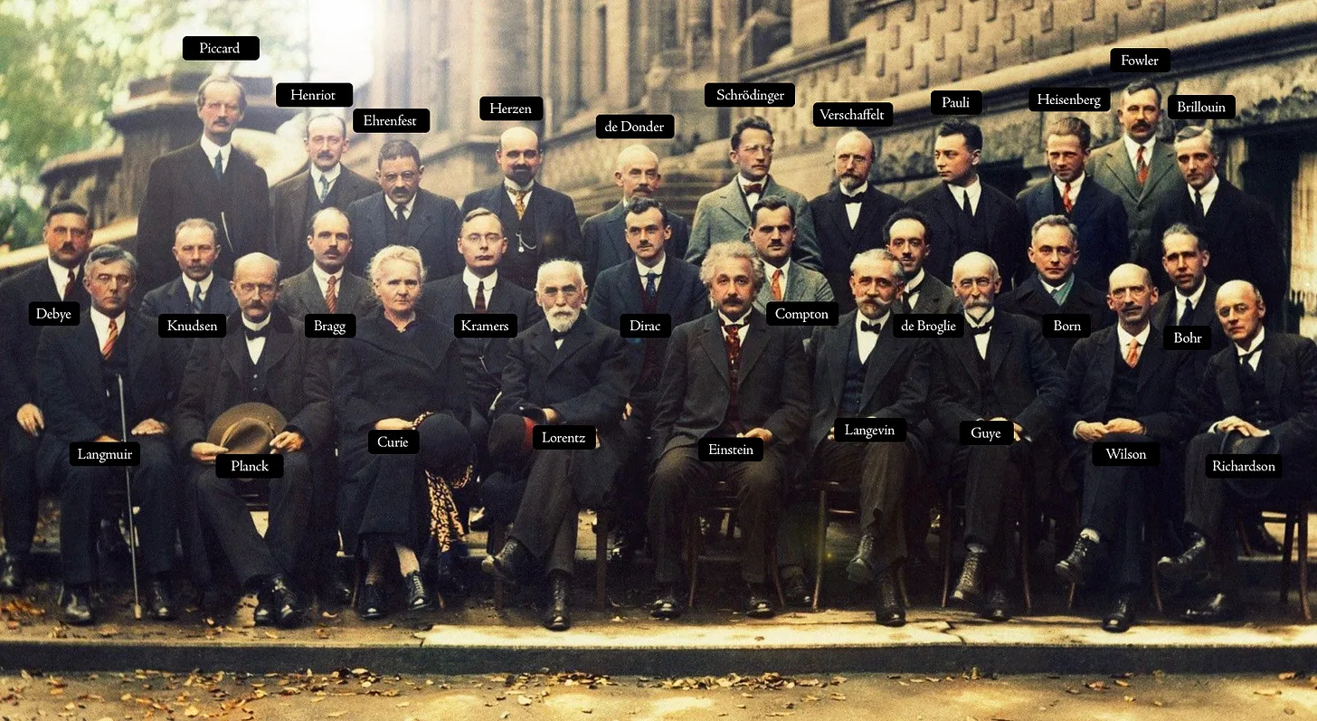
Photograph by Benjamin Couprie, Institut International de Physique Solvay, Brussels, Belgium.
Color: Marina Amaral
2.1 Lasers
2.2.1 Population Inversion
In the simple two-level energy systems we have considered so far, we may invoke the Boltzmann principle of thermodynamics. Having two energy levels, $E_1$ and $E_2$, with the populations, $N_1$ and $N_2$, respectively, the Boltzmann factor describes the population ratio:where $k_B = 1.380 \, 649 \cdot 10^{-23} \, \mathrm{J} / \mathrm{K}$ is the Boltzmann constant and $T$ is the temperature. The factor $g_2/g_1$ represents the degeneracy level, which is the number of allowed electrons in the upper state divided by the number of allowed electrons in the lower state. From this expression, we deduce that there are always more electrons in the lower energy state:
This is a consequence of stimulated emission in a two-level system, since the radiation at wavelength $\omega_{12} = \left( E_2 - E_1 \right)/\hbar$, causing the excitation of electrons, also stimulates decay.
To avoid this issue, we may consider a three-level energy system. In this case, we have three energy states $E_1 < E_2 < E_3$, such that $E_1$ represents the ground state. Imagine all the atoms initially in the ground state. Subjecting these atoms to a light source with frequency $\omega_{13} = \left( E_3 - E_1 \right)/\hbar$, causes some of them to excite into the upper state, $E_3$, a process referred to as pumping. Following excitation, the atoms will start to spontanuously decay to the second state, $E_2$. For laser operation, it is essential that the excited atoms decay quickly, i.e. the spontanuous emission lifetime, $\tau_{32}$, must be short. This energy transition may result in the emission of a photon, but often this transition is radiationless with the energy emitted as heat instead of radiation.
The atoms may then spontanuously decay once more to the ground state, $E_1$. In this case, it is desirable to release the energy as radiation in the form of a photon with frequency, $\omega_{21} = \left( E_2 - E_1 \right)/\hbar$. This transition is referred to as the laser transition. In the case that $\tau_{21} \gg \tau_{32}$, the population in the upper state, $E_3$, will essentially be zero, with atoms accumulating in state, $E_2$. This causes a population inversion, essentially meaning that $N_2 > N_1$.
To obtain population inversion in a three-level energy system, at least half the population of atoms must be excited from the ground state. This requires a large amount of energy, making three-level lasers rather inefficient. Instead, we may consider a four-level energy system, with energy states $E_1 < E_2 < E_3 < E_4$. In this system, rapid decay occurs for the transitions $E_4 \rightarrow E_3$ and $E_2 \rightarrow E_1$, while the in-between-transition, $E_3 \rightarrow E_2$, has a much longer decay time. This will cause atoms to accumulate in the $E_3$ energy state while essentially no atoms reside in the $E_2$ energy state. As a result, population inversion between the $E_2$ and $E_3$ states is accomplished, whithout needing to exicte a large number of atoms from the ground state, $E_1$.
What is so special about population inversion? - Optical amplification!.
2.2.1 The Resonator
2.2 Spectroscopy
2.3 Mach-Zehnder Interferometer
2.4 Corner-Cube Gravimeters
Part 3: The Second Quantum Revolution
The second quantum revolution is happening right now as new techonology and inventions are being developed. For this reason we are still not aware of the consequences of this second revolution. Whereas the first quantum revolution focused on using quantum mechanics to understand the processes around us, the second quantum revolution is about detecting and manipulating single quantum objects such as atoms, photons and electrons. For example, in the first quantum revolution we could explain the periodic table, but in the second quantum revolution we are learning how to build new atoms such as quantum dots and excitons, whoose properties we can engineer to our desire. This makes measurement accuracy at quantum scales possible.3.1 Techniques for Slowing and Cooling Atoms
A laser creates a collimated monochromatic light beam, which essentially means emitting a large number of photons along the same direction in space and with equal energy. If the energy of the photon, $E=\hbar\omega$, matches a tranisition between two energy states of the atom, $\triangle E=\hbar\omega_0$, the probablity of the atom absorbing the photon is maximized. Additionally, the photon carries a momentumwhere $\lambda$ is the laser wavelength. The rule of conservation of momentum implies that when an atom absorps a photon it experiences a slight "kick" in the direction of the incoming particle. The same "kick" is also experienced when the atom later decays back to the ground state, emitting another photon in a random direction. Since the emission occurs in random directions, the net "kick" following a large number of decays averages to zero. However, the incoming photon from the laser always acts in the same direction, effectively changing the atom velocity along the beam direction. The net effect is very similar to firing an arsenal of ping-pong balls onto a heavier bowling ball as illustrated in the animation below.
The net scattering force on the atom may be expressed as:
where $\sigma_\text{absorption}$ is the absorption cross section, which is a measure for the probablity of absorping a photon. This measure effectively depends on the detuning of the laser from atomic resonance, i.e. $\delta = \omega_0 - \omega$. The force also depends on the laser intensity, $I$, which is basically a measure of the number of photons encountered by the atom.
3.1.1 The Zeeman Slower
As the atom is moving towards the laser source, the wavelength of the laser beam is shifted in the observers reference frame according to the Doppler effect. For velocities much smaller than the speed of light, this effect may be expressed as:where $v$ is the atom velocity and $k = \omega / c$ is the laser beam wave number. In order to maximize the probability of absorption, one has to tune the laser wavelength to match the atom's transition energy. The opposite, namely modifying the transition wavelength of the atom to match the laser frequency is also possible. Additionally, since the atom continuously slows down, the transition wavelength must similarly change continuously to match the atom velocity. One way of accomplishing exactly this is based on the Zeeman effect that an ambient magnetic field changes the transition frequency of the atom by an amount $\left( \mu_B B \right) / \hbar$, with $B$ being the intensity of the magnetic field and $\mu_B$ the magnetic moment of the transition. Taking this effect into account, the resonance condition becomes:
where $\delta'$ is the effective detuning of the system. The Zeeman slower is thus constructed from a system of magnetic coils that results in a spatially varying magnetic field, $B (z)$, corresponing to the change in velocity, $v(z)$. The net effect is illustrated in the animation below.
One important feature of the Zeeman slower is that it works effectively for all atoms with an initial velocity below some threshold, $v_\text{max}$. At some point along the Zeeman slower, these atoms will satisfy the resonance condition and start slowing down. Atoms having an initial velocity above the threshold will never experience any effect of the Zeeman slower.
3.1.2 Optical Molasses
In the method of optical molasses, several laser beams are used to slow down the atoms. As argued previously, if the laser frequency, $\omega$, is in resonance with the transition frequency, $\omega_0$, between two energy states, $\left\vert \phi_1 \right>$ and $\left\vert \phi_2 \right>$, the atom will experience a net acceleration in the direction of the laser beam (away from the laser). For optical molasses, the laser is slightly detuned from the transition frequency, such that stimulated absoprtion in principle does not occur. In practice, however, the laser frequency spectrum will be some narrow bell shaped curve around the center frequency, meaning that some small degree of absorption will occur, resulting in a net acceleration along the laser beam. However, if two laser beams are placed in opposite directions along the same line, the net effect will be zero.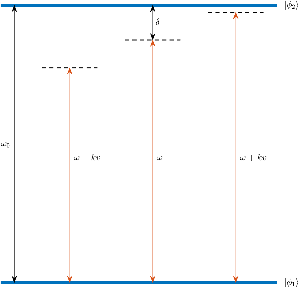
The laser wavelength, $\omega$, is slightly detuned from the transition frequency, $\omega_0$, between the two energy states $\left\vert \phi_1 \right>$ and $\left\vert \phi_2 \right>$ of the atom.
In the case that the atom is moving torwards one laser, it will experience a Doppler shift of the laser frequency, $\triangle \omega = k v$. As a result, the effective laser frequency, $\omega + k v$, will be closer to the resonance frequency of the energy transition, leading to a larger degree of stimulated absorption. This effectively slows down the atom as it moves against the laser beam.
In the case that the atom is moving away from the laser, the Doppler shift will have the opposite effect. The effective laser frequency, $\omega - k v$, will move further away from the transition frequency, $\omega_0$, having no net effect on the atom.
By using two counter-propagating laser beams, the atom can be effectively slowed down in both directions. For small velocities compared to the laser spectral width, i.e. $kv \ll \triangle \omega$, this force can be expressed as:
where $\alpha$ is the effective damping coefficient. The net effect is similar to that of a moving object being damped when submerged in a viscuous fluid. In the animation above, the principle is illustrated using two pairs of counter-propagating laser beams. Using three pairs of laser beams, this can be accomplished along all three directions in space.